Design and performance¶

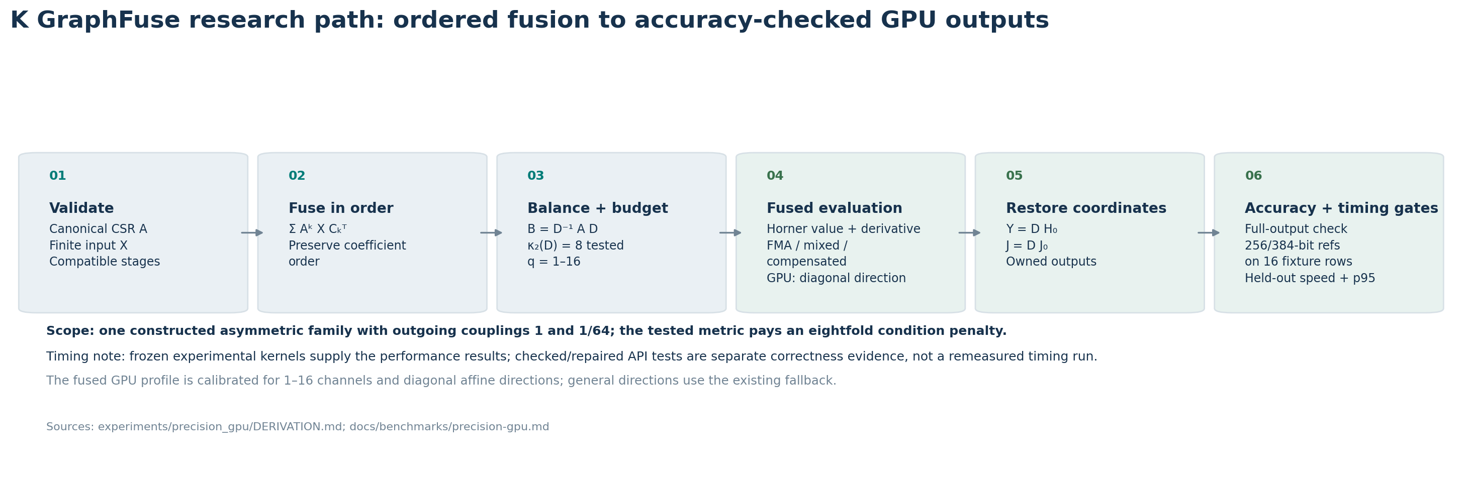
Ordered coefficient fusion, similarity scaling, sparse GPU evaluation and accuracy and timing checks

The figure describes the experimental precision path. The technical manuscript states its exact identities, conditional error transfer, implementation costs and measured scope.

Compile compatible stages¶

The compiler convolves channel coefficients in stage order using exact rational arithmetic. It computes geometry bounds and selects a retained degree under the requested budget. Exact cancellation can remove terms; conservative bounds or strict tolerances can retain the full degree. Fusion can also increase degree. It is not an optimal approximation across every polynomial representation.

Evaluate without graph powers¶

Sparse Horner evaluation uses repeated sparse matrix–dense state products and channel actions. With degree m, N_A stored entries and q channels, value evaluation costs O(m(N_A q+n q²)) arithmetic operations. Storage includes the sparse operator, n × q states and m × q × q coefficients. No dense n × n graph power is materialized.

Sensitivity evaluation couples the value with its derivative. It also uses a sparse direction E; its general cost is O(m(N_A q+N_E q+n q²)), up to fixed factors. Nonzero parameter values can add direction actions. The block lift in the derivation is a proof device and is not allocated by the evaluator.

These counts omit exact-rational bit-length costs. Compilation can be expensive and needs amortization. GPU packing can add workspace on the order of (m+1)nq; capture keeps persistent buffers. Diagonal and zero actions use cheaper operations when available, but the best configuration depends on the task.

Separate mathematical and engineering effects¶

The complete-inequality constant can tighten a tail certificate. Sparse execution, batching, precision, launch scheduling and CPU/GPU hardware can separately affect measured latency. The matched public PageRank experiment uses zero truncation and an unchanged finite polynomial. Its observed advantage is an implementation result on that workload, not evidence that a manuscript improved its degree.

The older sensitivity control includes a one-million-vertex case with degree 18 under K=2 and 19 under the older complete constant; observed resident time was approximately 242.49 versus 256.41 ms. Most other compared degrees were identical. Consult the raw candidate evidence before assigning gains to mathematical novelty.

Local propagation has a locality limit¶

prepare_local adds a CSC index. evaluate_local discovers nodes reachable within the retained degree and returns sparse COO output. The neighborhood can cover the whole graph; the implementation falls back to global evaluation after the selected set exceeds one quarter of vertices. It does not guarantee sublinear work on arbitrary graphs.

See API reference, mathematics and measurement methods.

Bound constants and discrete work¶

The bound-attribution analysis holds the backend, graph, inputs and budget fixed while changing the planner's numerical-range constant. Two of eleven legacy records lose one propagation stage; nine retain the same degree. This can reduce a constant amount of work without changing the asymptotic complexity. The 17.1573% value-tail factor reduction and 3.56–5.35% observed latency reductions are different quantities. The exact 9→8 GPU time remains unmeasured.