K GraphFuse: Similarity-Aware Sparse Polynomial Evaluation with Selective GPU Compensation

Utkarsh Sinha

Technical research manuscript / preprint draft, revised 11 October 2026; not peer-reviewed.

Download the PDF · Standalone LaTeX source · Metric definitions

Abstract

We study finite matrix-valued sparse polynomial actions and fixed affine directional sensitivities. K GraphFuse integrates condition-penalized dyadic similarity planning, ordered coefficients, fused Horner execution and selective compensation. The supporting transfer bound is elementary; balancing, graph polynomials and compensated arithmetic are prior art. The complete constant-two Crouzeix inequality is an attributed external premise, not re-proved here. The specific contribution is an inspectable integration and controlled empirical separation of its components, with no worldwide-first claim.

A publicly frozen repaired implementation is confirmed on six graph families, ten fixtures, two independent input/coefficient seeds per device and two GPU architectures. Additional packed-balanced CuPy controls are frozen before separate fresh-seed runs. Under matching original-coordinate budgets and matching selected degrees, 18/20 pooled device–fixture comparisons pass the strong speed gate, with 36.88–83.71% less resident compute time in those wins; R-MAT instead uses 55.52% more time on RTX and 2.21% more on T4. Every large output passes full FP64 CPU checks, with separate complete 64-row 256/384-bit checks. Same-backend comparisons show balancing can reduce degree 22 to 13, or increase degree 20 to 24 and slow execution.

A complete MovieLens 1M recommendation workflow preserves Recall@10, nDCG@10 and all top-10 lists. Against an algebraically equivalent specialized scalar-restart control, K uses 7.13% more pooled-median request time on RTX and practically ties T4; no end-to-end median speed gain is confirmed. Historical six-case T4 measurements and the separate native-cuGraph study remain distinct. This study does not compare these polynomial cases with native cuGraph, establish exhaustive SOTA, prove universal execution accuracy or change the installed K GraphFuse core.

A retrospective source-checked attribution of eleven earlier T4 workload records identifies two theorem-dependent degree reductions, 23→22 and 19→18. All eight accepted matching FP64 packing/capture configurations in those two cases record 3.56–5.35% less median time. Nine records retain the same degree. These are single-run observations; the exact CPU 9→8 boundary is untimed and the checked laptop constant comparisons have equal degrees. This demonstrates an application of the supplied theorem, without establishing worldwide-first algorithmic priority.

Keywords: sparse graph filters; matrix polynomials; similarity scaling; numerical range; Horner evaluation; directional sensitivity; compensated arithmetic; CUDA

1. Introduction

Many graph workloads apply a sequence of linear sparse propagations and small channel transforms to a feature matrix. When the graph operator is fixed and the stages are linear, the ordered stages can be represented by a single matrix-valued polynomial. Evaluation then becomes a sequence of sparse matrix–feature products plus dense transformations on a small channel dimension. This is a useful setting for fusing memory-bound sparse work while retaining the full finite polynomial.

This manuscript asks which gains come from coordinate changes, execution fusion and compensation under one original-coordinate accuracy requirement, and whether they survive a complete application. One deliberately asymmetric sparse family motivated the historical six-case experiment. The revised study freezes the repaired method before fresh confirmation across six families and two devices, then tests packed-balanced controls and a specialized application control in separately frozen follow-ups.

The results identify conditional kernel gains and practical counterexamples. Balancing lowers the degree on the alternating fixture but raises it on random sparse fixtures. R-MAT defeats the fused row-oriented executor. The real-data recommendation application preserves quality yet has no confirmed end-to-end median gain against an efficient scalar recurrence. This is a regime map for a specified computation, rather than a universal graph-processing claim.

The implementation remains separate from installed k_graphfuse 0.1.0. Historical results use source/product_v1 and source/wide_v1. New confirmations use current repaired sources pinned by studies/controlled_20261010/FREEZE.json. The initial environment failure, repair and excluded controls remain documented.

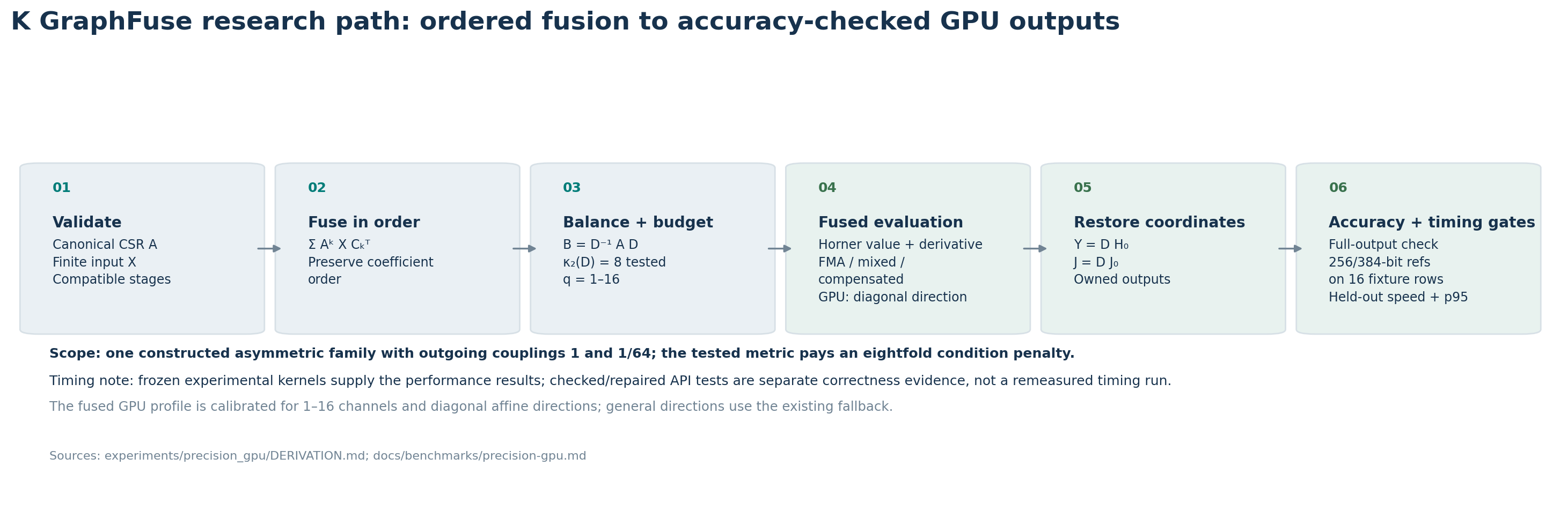
Figure 1. Pipeline overview.

1.1 Contributions

This manuscript documents four bounded contributions.

1. An inspectable integration of original-coordinate budget planning, finite ordered matrix-valued polynomial actions and fixed affine sensitivities with selective compensated CUDA execution.
2. Controlled component evidence with matching requested accuracy, identical execution backends where possible, retained-degree reporting, fixed profiles and fresh-seed two-device confirmation.
3. An isolated attribution of the supplied theorem's bound constant to retained degree and observed GPU time, with all matching execution settings and explicit CPU/laptop limitations.
4. A reproducible real-data recommendation workflow that tests complete request latency and held-out quality, including an efficient control that removes the apparent application speed advantage.

The specific contribution is an inspectable integration of original-coordinate error-budget planning for finite sparse matrix-valued polynomial actions and fixed affine sensitivities, with selective compensated CUDA execution, plus a controlled regime map that separates coordinate choice, execution fusion and compensation. The similarity transfer proof is elementary supporting analysis. Balancing, polynomial graph filters, Horner evaluation, error-free transforms and sparse fusion are established prior art. Worldwide first priority for this integration is unestablished.

2. Problem and notation

Let \(A\in\mathbb{R}^{n\times n}\) be the stored sparse operator and \(X\in\mathbb{R}^{n\times q}\) a feature matrix. Let \(C_k\in\mathbb{R}^{q\times q}\), \(k=0,\ldots,d\), be the exactly fused, ordered coefficient matrices. The target is

\[ P_A(X)=\sum_{k=0}^{d} A^k X C_k^{\mathsf T}. \]

The coefficient matrices need not commute. The polynomial representation therefore preserves the order induced by the original linear stages. Under row-major vectorization, the corresponding feature-space operator is \(\sum_k A^k\otimes C_k\), whose Euclidean norm induces the Frobenius norm on feature matrices. We measure value error in Frobenius norm, normalized by \(\|X\|_F\). This is not a per-vertex relative-error contract and is not aggregate PageRank \(L_1\) error.

For a fixed sparse direction \(E\), define \(A(\theta)=A+\theta E\) on a specified interval \(|\theta|\le h\), with \(C_k\) and \(X\) fixed. The directional sensitivity is

\[ J_A(X;\theta)=\frac{d}{d\theta}P_{A(\theta)}(X). \]

It is not an adjoint gradient or a nonlinear graph-learning derivative.

3. Similarity transform and error transfer

Choose a fixed positive diagonal matrix \(D\), and define \(B=D^{-1}AD\). Then \(A^k=DB^kD^{-1}\), so termwise

\[ P_A(X)=D\,P_B(D^{-1}X). \]

Right multiplication by \(C_k^{\mathsf T}\) does not alter the coordinate-change identity.

Theorem 1: transfer of a balanced-coordinate approximation bound

Suppose a linear evaluator \(\widehat P_B\) satisfies, for every \(Z\in\mathbb{R}^{n\times q}\),

\[ \|P_B(Z)-\widehat P_B(Z)\|_F\le \delta_B\|Z\|_F. \]

Define the original-coordinate evaluator \(\widehat P_A(X)=D\widehat P_B(D^{-1}X)\). Then

\[ \|P_A(X)-\widehat P_A(X)\|_F \le \kappa_2(D)\,\delta_B\,\|X\|_F, \qquad \kappa_2(D)=\|D\|_2\|D^{-1}\|_2. \]

Proof. The exact similarity identity gives

\[ P_A(X)-\widehat P_A(X) =D\left(P_B(D^{-1}X)-\widehat P_B(D^{-1}X)\right). \]

Apply \(\|DY\|_F\le\|D\|_2\|Y\|_F\), then the assumed bound with \(Z=D^{-1}X\), and finally \(\|D^{-1}X\|_F\le\|D^{-1}\|_2\|X\|_F\). Multiplying the factors yields \(\|D\|_2\|D^{-1}\|_2\delta_B\|X\|_F\). \(\square\)

Thus an original-coordinate normalized error budget \(\varepsilon\) requires a balanced-coordinate budget no larger than \(\varepsilon/\kappa_2(D)\). The result is independent of how \(D\) was selected. It applies to any operator-norm approximation bound satisfying the theorem’s hypothesis, including a truncation or coefficient-encoding bound. Floating-point execution error is additional unless separately bounded.

3.1 Numerical-range tail bound as a conditional premise

For a matrix \(B\), its numerical range is \(W(B)=\{u^*Bu:\|u\|_2=1\}\). Let \(Q_m(z)=\sum_{k=0}^{m}C_kz^k\) be the retained polynomial and let \(a_k\) upper-bound \(\|C_k\|_2\). If \(W(B)\) lies in an origin-centered disk of radius \(r\), a complete spectral-set inequality with constant \(K=2\) gives the conditional tail bound

\[ \left\|\sum_{k>m}B^k\otimes C_k\right\|_2 \le 2\sum_{k>m}a_k r^k. \]

A classical operator-norm enclosure \(\rho\ge\|B\|_2\) also gives \(\|\sum_{k>m}B^k\otimes C_k\|_2\le\sum_{k>m}a_k\rho^k\). The planner takes the smaller valid bound. The use of \(K=2\) takes the complete Crouzeix inequality in OpenAI manuscript 325-01 as an external theorem premise [3]. The proof of that premise was not independently rebuilt or checked for this manuscript. The similarity transfer in Theorem 1 is proved here; the heuristic choice of \(D\) does not change the theorem’s validity.

3.2 Implemented dyadic metric

Let \(r_i\) and \(c_i\) be the absolute off-diagonal row and column sums of \(A\). For indices where both are positive, the implementation sets

\[ e_i=\left\lceil\frac{\log_2(r_i)-\log_2(c_i)}{4}\right\rceil, \qquad D_{ii}=2^{e_i-\max_j e_j}. \]

If either sum is zero, it uses \(e_i=0\). This is one parallel balancing step. The exponent rule is heuristic and is not an iterative optimizer. The condition penalty is computed as \(2^{\max_i e_i-\min_i e_i}\). The transformed sparse entries are scaled by binary exponents and scaled back; nonfinite values, underflow, or failure of exact round-trip equality reject the transform.

In the tested alternating directed family, off-diagonal couplings are \(1\) and \(1/64\). The chosen scale alternates between \(1\) and \(1/8\), equalizing the two transformed couplings at \(1/8\). The resulting \(\kappa_2(D)=8\) incurs an eightfold error-budget penalty. The narrower balanced numerical-range enclosure nevertheless lets the planner retain fewer polynomial terms for this construction.

4. Coupled value and derivative evaluation

Hold \(D\) fixed while \(A(\theta)=A+\theta E\) varies. Write \(Z=D^{-1}X\), \(B(\theta)=D^{-1}A(\theta)D=B+\theta F\), and \(F=D^{-1}ED\). Then

\[ \frac{d}{d\theta}P_{A(\theta)}(X) =D\,\frac{d}{d\theta}P_{B(\theta)}(Z). \]

The value and derivative budgets are both divided by \(\kappa_2(D)\).

For retained degree \(d\), initialize \(H_d=ZC_d^{\mathsf T}\) and \(J_d=0\). For \(k=d-1,\ldots,0\), using the previous states before overwriting,

\[ J_k=B(\theta)J_{k+1}+F H_{k+1},\qquad H_k=B(\theta)H_{k+1}+ZC_k^{\mathsf T}. \]

Since \(H_d\) is independent of \(\theta\), \(J_d=dH_d/d\theta\). If \(J_{k+1}=dH_{k+1}/d\theta\), the product rule gives

\[ \frac{dH_k}{d\theta} =F H_{k+1}+B(\theta)\frac{dH_{k+1}}{d\theta} =F H_{k+1}+B(\theta)J_{k+1}=J_k. \]

Induction proves the recurrence at every degree, and the returned outputs are \(DH_0\) and \(DJ_0\). The recurrence preserves coefficient order and requires no commutativity assumption. For the tested diagonal direction with entries \(\pm1\), \(F=E\), so the directional product is elementwise. A general sparse \(F\) requires another sparse multiplication and uses the existing fallback path. Floating checks were made at \(\theta=0\) and both interval endpoints; those samples do not validate every floating output throughout the interval.

5. Coefficient encoding and arithmetic

For an exact rational coefficient matrix \(C_k\), let \(H_k\) be its elementwise round-to-nearest binary64 encoding. An optional low part is \(L_k=\operatorname{round}_{64}(C_k-H_k)\); high-only execution sets \(L_k=0\). Define the exact rational remainder \(R_k=C_k-H_k-L_k\), and let \(a_k\) be an exact rational upper bound on \(\|R_k\|_2\). If \(\rho\ge\|B\|_2\) and \(W(B)\) lies in a disk of radius \(r\), the encoded-polynomial error obeys

\[ \left\|\sum_k B^k\otimes R_k\right\|_2 \le \min\left\{\sum_k a_k\rho^k,\quad 2\sum_k a_k r^k\right\}. \]

The original-coordinate bound multiplies this by \(\kappa_2(D)\). The derivative’s encoding error is bounded separately by the existing directional-derivative polynomial bound, with the parameter interval included in its operator and numerical-range enclosures. These bounds account for exact polynomial truncation and coefficient representation. They do not account for CUDA execution roundoff, overflow, or underflow.

The narrow CUDA kernel assigns work to row/channel outputs and combines CSR edge accumulation, coefficient injection, and (when requested) the directional derivative. It uses alternating state buffers. FMA-based, compensated, mixed, and double-double profiles are available in the experimental source. Plain FMA uses one rounding for a product-plus-sum. Compensation tracks product and addition residuals; the compensated profile still rounds completed per-thread sums at stages. No profile eliminates all rounding or removes overflow and underflow risk.

For wide features, a BLAS projection forms \(ZC_k^{\mathsf T}\) terms into dense workspace before sparse Horner evaluation. The 16-channel profile uses high-only coefficient projection and a separately compiled compensated final step. It trades extra projection workspace for throughput; it does not establish memory savings against every comparator.

For degree \(d\), \(m\) stored nonzeros, \(n\) vertices, and \(q\) channels, the stated arithmetic work is \(O(dm q+d n q^2)\). Narrow resident storage is \(O(m+nq+dq^2)\), including the sparse operator, scales, coefficients, and reused states. Wide projection adds \(O(dnq)\) workspace. These are constant-factor and memory-traffic optimizations; the asymptotic graph-work bound is unchanged.

6. Relation to prior work

Polynomial evaluation, sparse Horner recurrences, exact ordered fusion of linear stages, and diagonal similarity are established ideas. Classical matrix balancing, including LAPACK’s DGEBAL routine, is important prior art [1]. K GraphFuse’s fixed, sparse, dyadic row/column heuristic differs from a dense iterative balancing routine and carries no optimality claim.

Crouzeix and Palencia established a complete \((1+\sqrt{2})\)-spectral-set bound for the numerical range [2]. A bivariate extension connects related estimates to Fréchet derivatives of matrix functions [4]. The current planner uses the constant-two complete inequality from OpenAI manuscript 325-01 as its stated premise [3]. OpenAI manuscript 325-02 motivates optimal similarity/positive-metric formulations; this implementation does not compute that optimal metric or transfer its condition bound to the heuristic diagonal scaling [5]. A separate OpenAI manuscript on the matrix multiplication exponent is not implemented and implies no finite-T4 speed result [6].

FMA semantics and the effects of floating-point operation order follow standard floating-point behavior documented by NVIDIA [7]. Compensation and mixed precision are execution choices, not exact-arithmetic certificates. The specific combination and performance behavior reported here are evaluated only under the experiment below.

The focused closest-method review compares LAPACK DGEBAL [1], balancing failure analysis [9], tolerance-selected exponential actions [10], polynomial graph filtering and channel mixing [11], linear graph-layer simplification [12], compensated Horner [13], GE-SpMM [14], FusedMM [15] and vendor sparse primitives [16]. These establish that balancing, degree selection, graph-polynomial representations, compensation and sparse fusion are existing ideas. Exponential actions have a different function target; GE-SpMM is a GPU sparse primitive, while FusedMM's published kernels are CPU-oriented. Chebyshev graph filters already use recursive sparse polynomial evaluation with channel weights. Those specific implementations and DGEBAL were not run as equivalent performance controls, so no superiority claim against them is made.

The specific contribution is an inspectable integration of original-coordinate error-budget planning for finite sparse matrix-valued polynomial actions and fixed affine sensitivities, with selective compensated CUDA execution, plus a controlled regime map that separates coordinate choice, execution fusion and compensation. The similarity transfer proof is elementary supporting analysis. Balancing, polynomial graph filters, Horner evaluation, error-free transforms and sparse fusion are established prior art. Worldwide first priority for this integration is unestablished. See the closest-method comparison for the exact distinctions and evidence gaps.

7. Historical experimental design

7.1 Constructed family

The experiment uses one constructed asymmetric sparse family at \(n=10^4,10^5,10^6\), with \(q=4\) and a separate \(n=10^5,q=16\) case. The operator has alternating diagonal entries \(-0.2\) and \(-0.1\) and alternating asymmetric directed couplings \(1\) and \(1/64\). The selected \(D\) alternates \(1\) and \(1/8\), giving \(\kappa_2(D)=8\). Each case uses a degree-48 matrix polynomial with geometrically decaying rational coefficients. Sensitivity cases use \(E\) diagonal with alternating \(\pm1\) and parameter interval \([-1/64,1/64]\). Their timings replay \(\theta=0\); the sensitivity accuracy checks additionally include both interval endpoints.

This is a deliberately chosen synthetic family. The six cases are related sizes and feature widths of the same construction, not six independent graph families.

7.2 Sources, controls, and profiles

The main timed implementation is frozen as source/product_v1; the separate wide follow-up is source/wide_v1. The baseline controls use a \(10^{-8}\) compiler truncation target, the similarity-aware main plans target \(10^{-16}\), and the high-only wide profile targets \(10^{-15}\). The controls are FP64 CuPy 14.2.0 and PyTorch 2.11.0+cu128 on the same Tesla T4, independently tuned for packing and graph capture where supported. Fourteen configurations were recorded per main case and eight in the wide follow-up.

Seven pilot samples per configuration preceded five randomized held-out confirmation blocks of 31 synchronized samples per selected method. The fastest accuracy-eligible pilot profile was selected; the comparison denominator is the fastest accepted held-out control. The selection policy and public \(10\%\) latency threshold were reconstructed after exploratory results, and the wide follow-up followed earlier wide-profile losses. This creates selection bias not represented in the intervals.

The selected profiles were fused FMA for the narrow value-only cases, mixed value/derivative compensation for the 100,000-vertex sensitivity case, full compensation for the million-vertex sensitivity case, and BLAS projection with a compensated final step for the 16-channel value case. Selection is hardware- and workload-specific, not a universal dispatcher.

7.3 Accuracy and speed gates

For each sampled value/derivative output, the accuracy screen requires every recorded Frobenius and maximum-absolute error component to be no worse than the fastest accepted control, with at least one component better. The reported “largest Frobenius component reduction” is a summary of sampled numerical errors, not a per-vertex or model-quality improvement. The speed gate requires at least \(10\%\) lower pooled median latency, the lower endpoint of the reported block interval above one, and p95 no worse.

The pooled-median ratio is the ratio of medians from all 155 held-out samples. The reported interval instead bootstraps the ratio of median block medians. These estimators differ; the interval need not contain the pooled-median ratio. Five blocks from one run characterize within-run variation, not cross-run or cross-device uncertainty, and the interval is not corrected for profile selection.

Timing is resident validated-input compute, including the owned GPU output and input/output similarity scaling. It excludes validation, host transfer, compilation/JIT and preparation. No isolated peak-memory, energy, end-to-end application, or cloud-bill measurement was made.

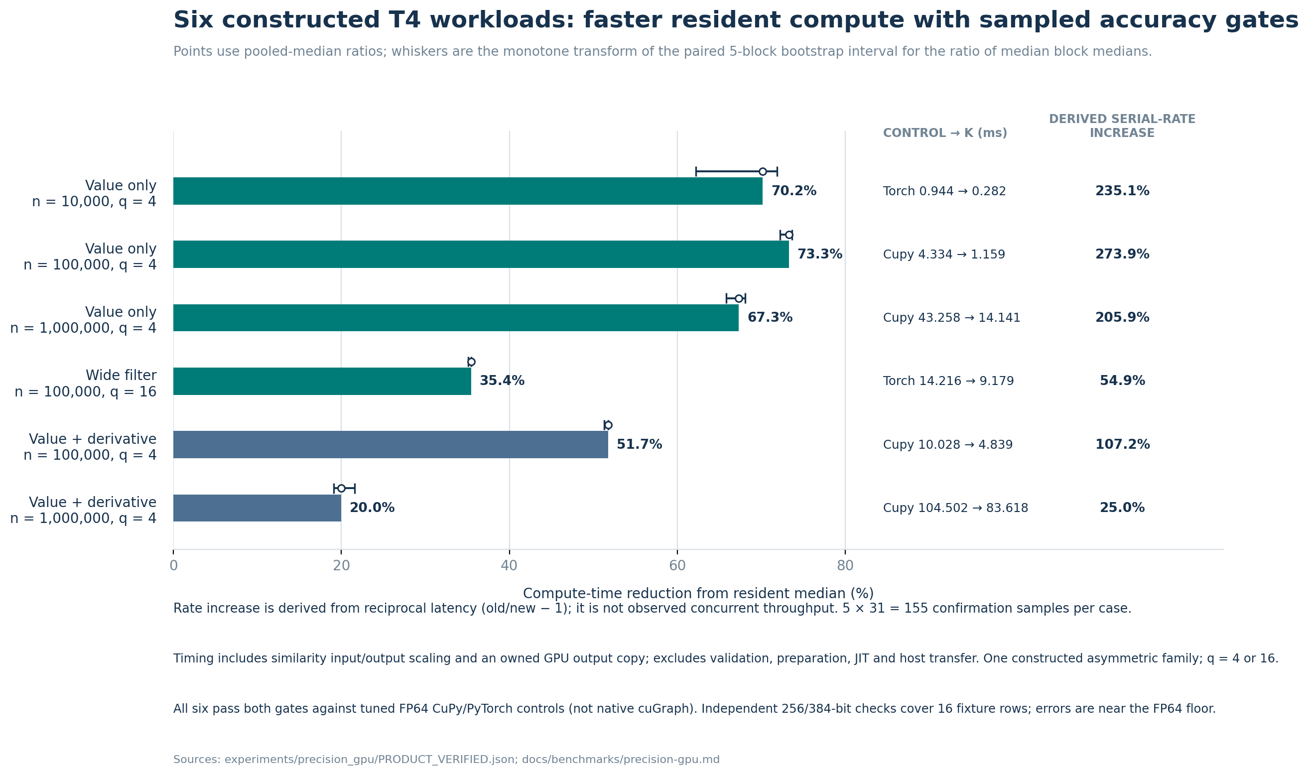
Figure 2. Latency reductions and reciprocal-latency rate changes.

8. Historical results and new controlled confirmation

All six selected T4 cases passed the recorded combined gates against their fastest accepted FP64 CuPy or PyTorch controls. The rate-change column is calculated as control median divided by K median, minus one. It is a reciprocal-latency transformation of the timing result, not a separate measured system-throughput result. See metric definitions for the formulas and interpretation.

Workload	Selected profile / control	Control median (ms)	K median (ms)	Latency reduction	Reciprocal-latency rate increase	Median ratio (block 95% interval)	Control / K p95 (ms)
10k × 4, filter	FMA / PyTorch	0.944	0.282	70.16%	235.12%	3.35× (2.65–3.55)	1.057 / 0.400
100k × 4, filter	FMA / CuPy	4.334	1.159	73.26%	273.95%	3.74× (3.60–3.79)	4.369 / 1.300
1M × 4, filter	FMA / CuPy	43.258	14.141	67.31%	205.91%	3.06× (2.93–3.13)	44.172 / 15.176
100k × 16, filter	Wide final / PyTorch	14.216	9.179	35.43%	54.88%	1.55× (1.54–1.55)	14.336 / 9.290
100k × 4, value + derivative	Mixed / CuPy	10.028	4.839	51.75%	107.24%	2.07× (2.05–2.07)	10.109 / 4.888
1M × 4, value + derivative	Compensated / CuPy	104.502	83.618	19.98%	24.98%	1.25× (1.24–1.28)	106.124 / 85.518

All pooled-median ratios meet the \(10\%\) reduction threshold; all interval lower endpoints exceed one and all selected p95 values are lower. The ratios and intervals are rounded from the audited PRODUCT_VERIFIED.json record.

Every full output was checked against degree-48 FP64 CPU evaluation; normalized differences were at most \(10^{-13}\). That CPU comparison covers all output entries but is itself rounded. Independent 256- and 384-bit sparse Horner references checked the first 16 rows for large fixtures using 64- and 128-row influence windows; those windows agreed below \(10^{-65}\). The finite influence-cone argument supports those sampled rows only. It does not establish arbitrary-precision truth for every output row or for other operators.

The sampled errors were near the FP64 floor. The largest sampled Frobenius component decreased by \(0.0077\%\), \(1.9316\%\), \(10.0281\%\), \(1.4723\%\), \(28.7375\%\), and \(19.9051\%\), respectively, in table order. Such small absolute errors mean a relative percentage can be numerically noticeable without implying a material downstream application gain. In the million-vertex sensitivity case, a faster mixed profile failed an error component; the selected fully compensated profile was slower but passed the screen.

8.1 Frozen controlled confirmation

The primary protocol fixes a degree-32 polynomial, rational channel matrices with geometric decay, a single original-coordinate truncation budget of 1e-12, and an additional 1e-13 empirical rounding-screen allowance. This screen is not a floating-roundoff proof. The six families are alternating asymmetric, already balanced, grid, random sparse, R-MAT and randomly similarity-scaled random operators. Ten fixtures vary size, 4/16 channels and two value-plus-derivative cases. Sensitivity timings/checks here use theta=0; interval planning remains conditional.

The fixed K profile is fused_onepass_captured, with current repaired sources pinned in FREEZE.json. The primary comparison includes six identity-coordinate FP64 CuPy/PyTorch controls with packing and supported capture. Twelve total methods isolate identity/one-pass/eight-sweep coordinates, identical-plan fusion, and compensation. The eight-sweep control uses simultaneous dyadic updates; it is Osborne-inspired and does not reproduce LAPACK DGEBAL's sequential algorithm. No optimal balancing claim is made.

Primary seeds 20261011/12 run in separate processes on RTX 3060 Laptop and Tesla T4. Five randomized paired blocks contain 11 synchronized resident samples per method per process, after three warmups. Owned outputs and original-coordinate scaling are included; validation, compilation, preparation and transfer are separate. Every large output is checked against a full finite-polynomial FP64 CPU reference. Every row of separate 64-row, four-channel fixtures across all six families is checked against 384-bit references cross-checked at 256 bits (discrepancy below 1e-65). These small checks do not certify every large row at arbitrary precision.

During review, packing combined with balancing was identified as a stronger compatible control. A separate public CONTROL_FREEZE.json fixes that follow-up before fresh seeds 20261013/14. It compares packed one-pass and packed eight-sweep CuPy with the same fixed K profile. All selected control/K retained degrees match in that confirmation. It was not part of the original freeze and is reported separately.

Point estimates and 95% intervals use the same pooled-median control/K ratio estimator. The analysis resamples paired whole blocks within each separate process, with 2,000 bootstrap draws and a fixed analysis seed. Intervals are descriptive, conditional on the observed fastest accepted control, and not multiplicity-adjusted. Pooling two coefficient/input seeds is a descriptive summary; it is not 110 independent graph observations. A strong speed gate requires at least 10% less median time, interval lower endpoint above one and no p95 regression.

The primary study passes the strong speed gate in 18/20 pooled device–fixture comparisons. The stronger packed-balanced confirmation also passes 18/20, with 36.88–83.71% lower pooled-median resident compute time in those 18 wins. The remaining R-MAT comparison uses 55.52% more time on RTX and 2.21% more on T4. Ten fixtures times two devices form these 20 comparisons; they are not 20 independent graph families.

The primary study has 40 case-runs, 480 large method checks and 288 small whole-fixture method checks. The follow-up has another 40 case-runs and 120 large method checks; these reuse the ten graph fixtures with fresh coefficients/inputs. Every recorded healthy large and small method passes the matching screen. The largest K full-output normalized FP64 CPU difference in the primary aggregate is 1.416e-14.

Balancing reduces the alternating q=4 value degree from 22 to 13 with condition penalty 8, giving 36.47% less T4 time on the same eager fused executor. In the random q=4 fixture it instead raises degree 20 to 24, causing 18.69% more T4 time on that executor. Balanced/grid/full-degree fixtures have no degree reduction. Fusion gains therefore remain distinguishable from coordinate gains. The compensated control uses 1.50–6.05 times the latency of the otherwise matching eager fused profile across the 20 pooled cases; the worst-of-two-seeds normalized CPU difference is no worse in only 6/20. These near-floor rounded-reference differences do not establish universal accuracy superiority or a compensated execution theorem.

T4 value-only fixture, q=4	Identity / one-pass degree	Condition penalty	One-pass time reduction on the same fused executor
alternating	22 / 13	8	+36.47%
balanced	30 / 30	1	-0.11%
grid	15 / 15	1	+0.24%
random	20 / 24	2	-18.69%
rmat	32 / 32	64	-0.70%
similarity random	32 / 32	64	-0.23%

Figure 3. Fresh-seed matched-degree confirmation; negative outcomes remain visible.

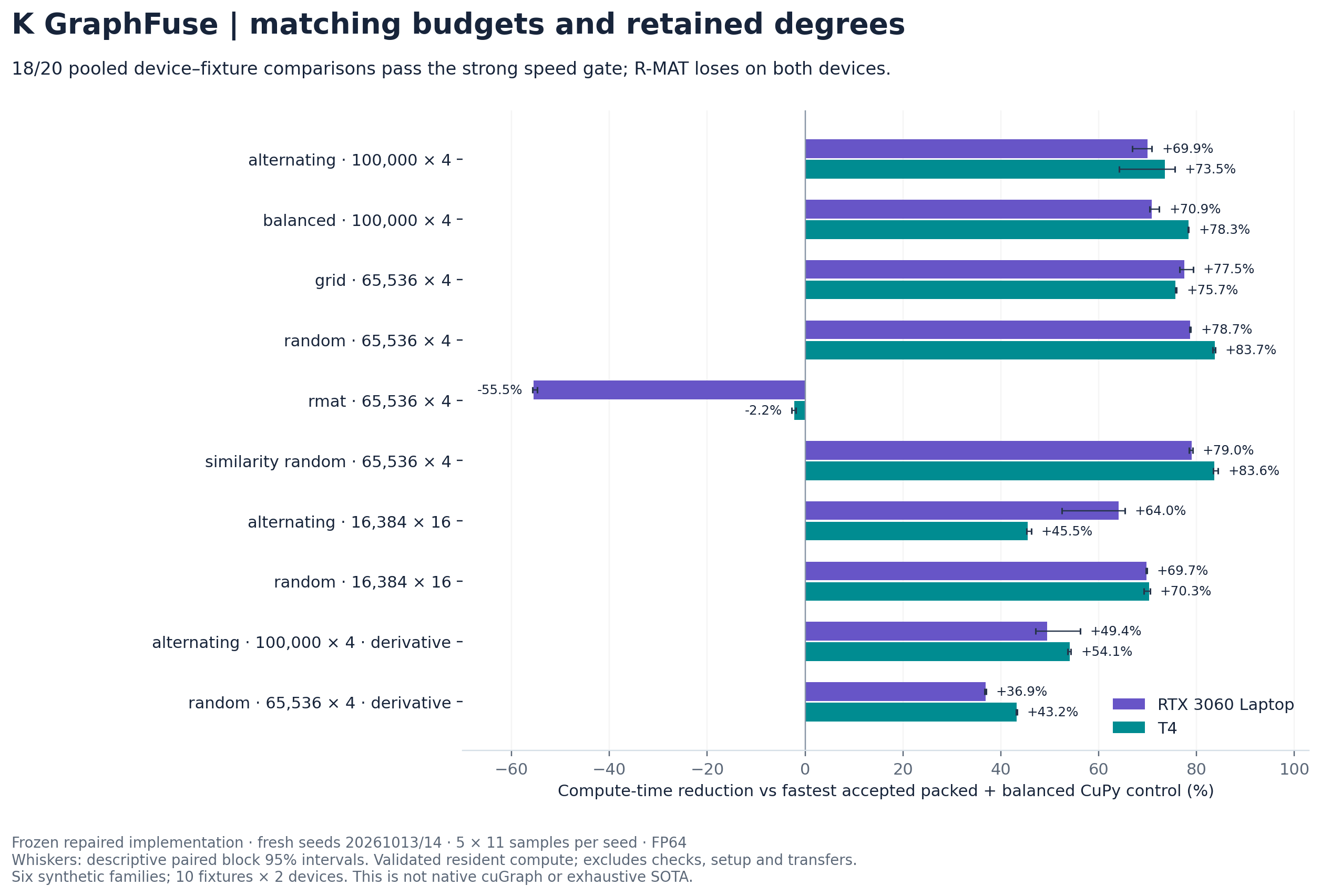
The packed-balanced control set isolates matching degrees; it does not replace the primary PyTorch competitor set or claim to be the fastest of every combined framework method. All 20 rows in each study, all 120 component comparisons, full error screens and intervals are in the controlled report and its hashed raw artifacts. These comparisons are separate from native-cuGraph PageRank.

8.2 Real-data recommendation application

The application is a reproducible MovieLens 1M recommendation workflow on real public ratings. Latest 20% of each user's timestamp-ordered ratings are held out. The training bipartite graph uses ratings >=4; all previously rated items are excluded from recommendations. There are 9,992 stored vertices, 944,258 stored positive-training edges and 256 deterministic eligible evaluation users, batched in four channels. The finite diffusion uses alpha=17/20 and degree 12. This is a fixed numerical recommender, not a trained recommendation quality-SOTA model.

Request timing includes seed construction, host-to-device transfer, checked numerical execution, device-to-host output, seen-item exclusion and stable top-10 ranking. Data load/graph construction, compilation and GPU preparation are recorded separately. APPLICATION_FREEZE.json fixes the stronger scalar-restart control before its separate runs: y0=(1-alpha)X, y[j+1]=alpha A y[j]+(1-alpha)X. This is algebraically the same finite polynomial, avoids unnecessary channel GEMMs, and receives the same finite input/output checks. Method order is shuffled within five whole-workflow blocks. All blocks remain recorded.

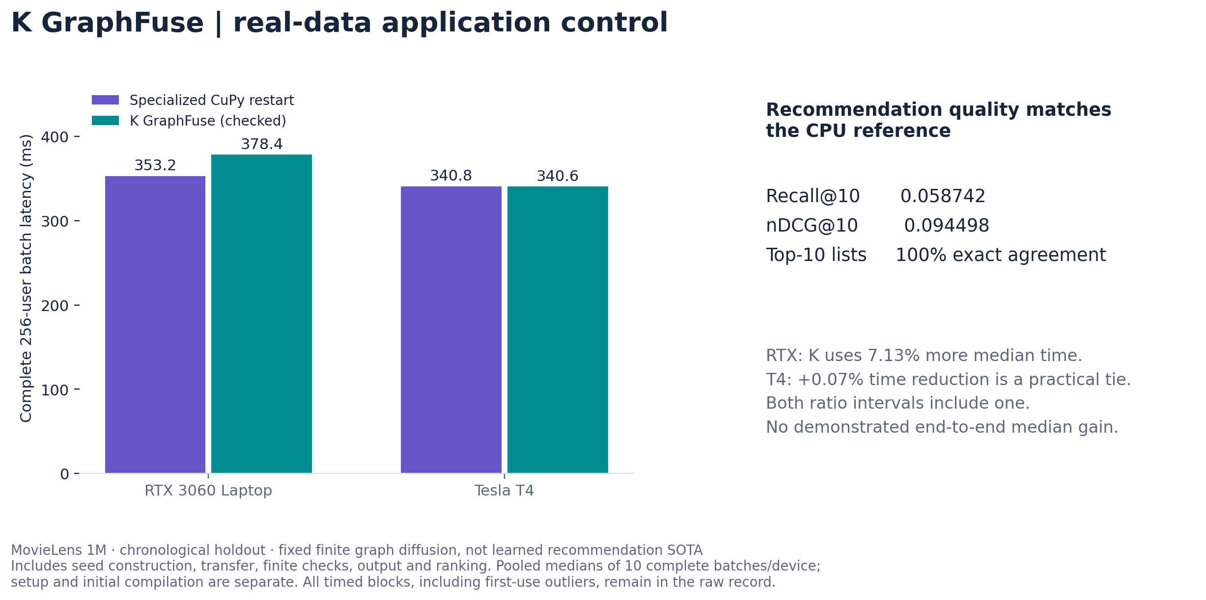
All healthy implementations have Recall@10=0.0587420862, nDCG@10=0.0944984887 and 100% exact top-10 agreement with the CPU finite-polynomial reference. The predeclared 0.001 absolute quality noninferiority margin passes. This demonstrates preserved application outcomes, not increased recommendation quality or relevance.

Against that specialized control, K uses 7.13% more pooled-median time on RTX and is a practical tie on T4 (+0.07% time reduction). Both descriptive ratio intervals include one. There is no confirmed end-to-end median speed advantage. The generic matrix-coefficient application controls in the primary raw runs are weaker; their apparent gains are not the application headline.

The observed application p95 values include a large first-use CuPy outlier in each first-seed process. Some lazy compilation happens inside the first request, while other preparation happens before timing, and cache state is not reset uniformly. Those observed tails are retained but do not establish superior steady-state tail latency or a fair fully cold comparison. Compile/preparation fields are the last reported warm-cache setup, not a cold-start distribution. No cold-start break-even or customer-cost saving is established. Captured CuPy restart fails with NotImplementedError on both devices and is an unsupported control, not a K win.

The archive SHA-256 is a6898adb50b9ca05aa231689da44c217cb524e7ebd39d264c56e2832f2c54e20. Only ratings are parsed; demographics and the archive are not redistributed. GroupLens research-use terms apply separately; commercial use requires their permission. Cite Harper and Konstan, The MovieLens Datasets: History and Context, ACM TiiS (2015), doi:10.1145/2827872.

GPU	Specialized CuPy / K median (ms)	Time reduction	Ratio (95% interval)	Observed CuPy / K p95 (ms)
RTX 3060 Laptop	353.198 / 378.386	-7.13%	0.933× (0.915–1.192)	4668.271 / 422.594
T4	340.838 / 340.595	+0.07%	1.001× (0.992–1.186)	5668.892 / 411.505

Figure 4. Complete recommendation request latency and quality parity.

8.3 Separate native PageRank context

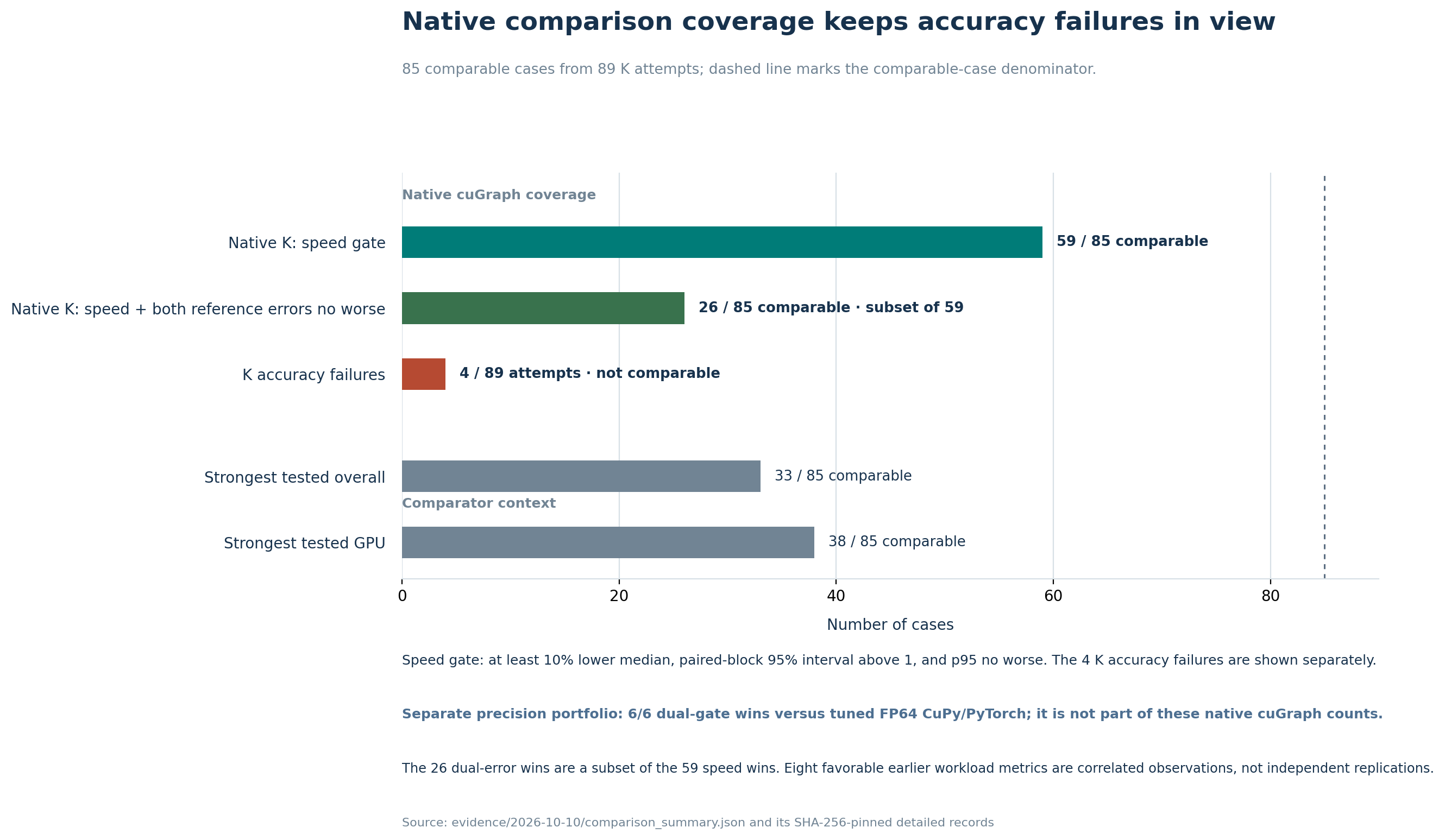
The precision experiment has no native-cuGraph control. A separate K GraphFuse PageRank/ranking study used different source, operators, error contracts, and candidate pools; it must not be pooled with the six cases above. That study records 15 suites, 111 records, 2,190 configurations, and 104 predeclared cases. Of 89 attempted native comparisons, 85 were comparable and 4 K cases lacked accepted accuracy. A strong speed gate passed in 59/85 comparable cases (59/89 attempts when failures count as non-wins); 26/85 comparables (26/89 attempts) also had aggregate \(L_1\) and maximum-relative errors no worse. The strongest-tested-control counts were 38/85 for GPU and 33/85 overall, including measured CPU alternatives. These denominators and gates belong only to that study.

The separate study also has losses: native cuGraph was 2.72× faster on Graph500-22; the later datagen confirmation measured K at 56.089 ms versus 54.667 ms for native; and full file-import and changing-graph rebuild workflows favored native cuGraph. The earlier 19-workload suite passed zero strongest GPU gates under its protocol. K GraphFuse does not implement BFS, SSSP, connected components, triangle counting, or Louvain. The native context provides scope and negative evidence, not corroboration of the precision-GPU results.

Figure 5. Coverage of the separate native-comparison study.

8.4 Isolated theorem-bound attribution in earlier runs

This analysis uses existing 10 October 2026 Tesla T4 runs, re-examined on 11 October. Authenticated read-only access checked ten completed relevant Kaggle kernels and retrieved thirteen JSON outputs. The two degree-changing cases and every candidate sample exactly match the already published raw records. No new GPU timing was generated.

The immutable source constructs both plans from the same stored operator, feature matrix, rational coefficient matrices, error budget and affine direction/interval where applicable. It changes only the complete-bound constant: older 1+sqrt_upper(2) versus default 2. Both plans use the same PyTorch evaluator. FP64 pairs match packing and CUDA capture. All four execution settings are retained; rejected FP32 settings are excluded. Source manifests and encoded run sources are audited without executing the GPU code.

The examined matrix-filter/sensitivity records contain eleven workloads. Two change retained degree and nine do not. The eight timing pairs are four configurations of each degree-changing workload, not eight independent graphs. Each configuration has 31 consecutive synchronized samples; configuration order is shuffled. There is no paired repeated-block or independent-repeat interval for these measurements. The extraction is retrospective; it is not a newly predeclared confirmation experiment.

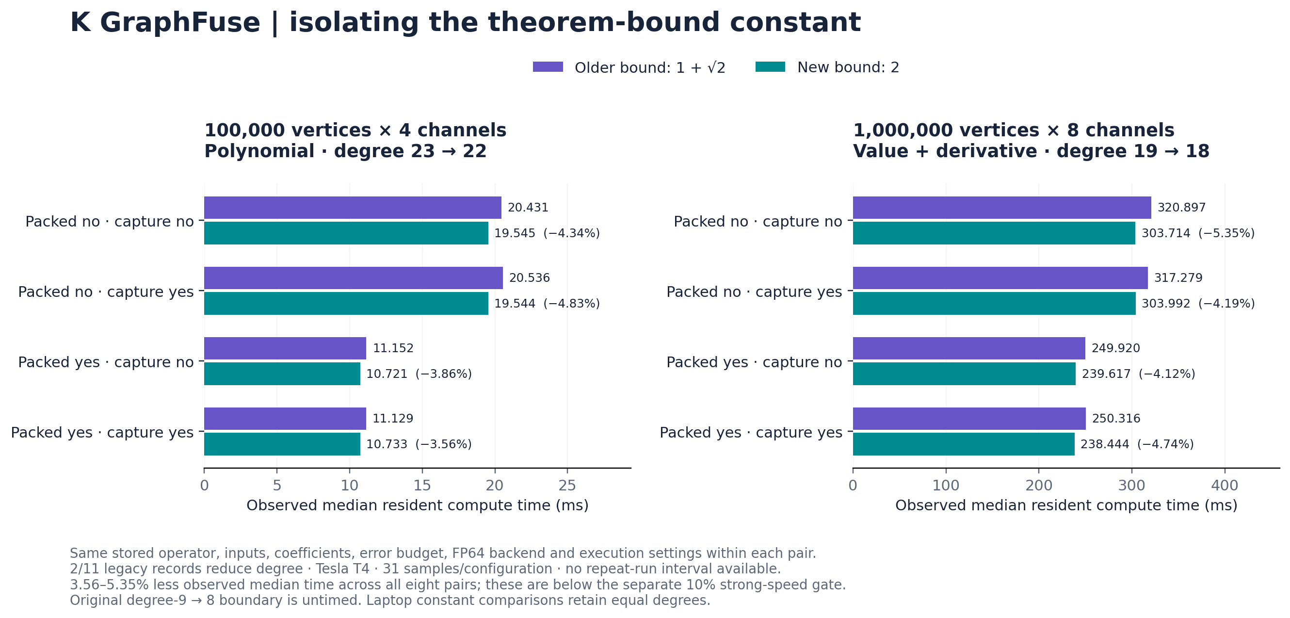
Among the eleven examined legacy workload records, two reduce degree and nine do not. The polynomial changes 23→22 at 100,000 vertices/four channels/budget 1e-12; the value-plus-derivative case changes 19→18 at one million vertices/eight channels/budget 1e-8. All eight accepted matched FP64 configurations in those two cases record 3.56–5.35% less median resident time and lower observed p95. These are below the separate 10% strong-speed threshold and add no native-cuGraph wins.

Workload / FP64 setting	Degree old → new	Old / new median (ms)	Less time	Old / new p95 (ms)
Polynomial 100k × 4; packed=False, capture=False	23 → 22	20.431 / 19.545	4.34%	22.789 / 20.017
Polynomial 100k × 4; packed=False, capture=True	23 → 22	20.536 / 19.544	4.83%	20.963 / 19.829
Polynomial 100k × 4; packed=True, capture=False	23 → 22	11.152 / 10.721	3.86%	11.534 / 11.041
Polynomial 100k × 4; packed=True, capture=True	23 → 22	11.129 / 10.733	3.56%	11.239 / 10.812
Value + derivative 1M × 8; packed=False, capture=False	19 → 18	320.897 / 303.714	5.35%	321.765 / 304.441
Value + derivative 1M × 8; packed=False, capture=True	19 → 18	317.279 / 303.992	4.19%	318.643 / 304.581
Value + derivative 1M × 8; packed=True, capture=False	19 → 18	249.920 / 239.617	4.12%	250.566 / 240.175
Value + derivative 1M × 8; packed=True, capture=True	19 → 18	250.316 / 238.444	4.74%	250.619 / 238.739

For the same nonzero value-tail residual, the factor change from 1+sqrt(2) to 2 tightens that numerical-range certificate by 17.1573%. A planner may retain fewer terms under the same budget; the ordinary norm branch or a discrete degree threshold can leave degree unchanged. This factor percentage is not a speed or universal floating-accuracy percentage. All listed outputs pass the same recorded FP64 CPU reference gate; their complete normalized differences are in the attribution report.

The CPU sparse record already demonstrates a degree-only boundary: older complete bound 9, new complete bound 8, ordinary norm bound 10, at selected tolerance 2.8361371852467578e-05. This boundary deliberately crosses a degree threshold. It contains no latency samples.

For the RTX 3060 Laptop GPU's six explicit old/new-constant cases, the recorded degrees match: 15/15 for four-channel polynomial cases, 16/16 for the sixteen-channel case and 18/18 for value-plus-derivative cases. Their similarity-aware degrees of 9 or 10 involve a coordinate change and cannot be relabeled as a constant-only 9→8 comparison. A literal degree-9-versus-8 GPU time, or an isolated laptop degree-changing time, remains absent from the checked records.

The stronger theorem is attributed to OpenAI. K GraphFuse's supported contribution is a computational application: an explicit truncation planner and inspectable integration, with evidence that the strengthened bound can remove a propagation stage and reduce observed GPU time on the stated inputs. This sharpens the research-paper contribution beyond aggregate benchmark gains. Worldwide-first application, a fundamentally new general algorithm and global SOTA remain unestablished. The similarity-transfer proof is supporting elementary analysis; it is not the source theorem.

The comparison changes the implemented general bound. It does not rule out sharper preexisting class-specific bounds for these operators; that review is required before claiming the new general theorem was necessary to certify the tested inputs.

Figure 6. All matched theorem-constant timings; no repeat-run intervals are inferred.

9. Limitations and threats to validity

Workload coverage. Historical six-case results use one constructed family. New confirmation covers six synthetic families, ten fixtures, two fresh coefficient/input seeds per phase and two devices. MovieLens adds one real-data fixed-model application. These are targeted numerical workloads, not broad graph-algorithm or production coverage.

Selection and uncertainty. Historical profile selection follows exploration. The new repaired profile/protocol is publicly frozen before confirmation. Packed-balanced and scalar-restart controls were identified during review and separately frozen before fresh confirmation, rather than being retrospectively folded into the initial protocol. Bootstrap intervals use paired blocks and the same pooled-median estimator; they are descriptive and do not adjust multiple comparisons or observed control selection. Both devices remain author-controlled. The retrospective theorem-bound attribution selects the two of eleven legacy records where degree changes and retains all four accepted FP64 execution settings; it has 31 consecutive samples per configuration, without paired repeated-block uncertainty or independent replication.

Accuracy and certificate scope. Large references are FP64 CPU arithmetic. Historical high-precision checks sample the first 16 rows; new high-precision checks cover whole separate 64-row fixtures. Neither proves every large output at arbitrary precision or every input/parameter. The additional rounding-screen allowance is empirical. The complete constant-two Crouzeix result is a pinned external premise. The elementary transfer proof and exact coefficient bounds do not bound execution roundoff, and dyadic balancing is heuristic.

Timing and application scope. Resident timings exclude setup, transfers and finite checks; separate checked-call samples are retained. The new application includes the full request path and separately records data construction and preparation. First-use compilation/cache differences prevent fair cold-start or steady-state tail conclusions from its observed p95. No customer saving, integrated energy, allocator-peak comparison or concurrent capacity was measured. A real application with unchanged quality and no confirmed median speed gain is a substantive limit on adoption claims.

External validity and priority. DGEBAL, GE-SpMM, FusedMM and Chebyshev/Clenshaw executors remain unmeasured as equivalent controls. No new balancing theorem, globally optimal metric, exhaustive SOTA, worldwide-first integration, peer review or independent external replication is established. The separate PageRank studies retain their own recorded losses and errors.

10. Applications and adoption criteria

The best-fit hypotheses are repeated low-channel sparse linear graph filters, asymmetric diffusion-style polynomials, and repeated sensitivity evaluations with a diagonal node parameter. A candidate application should first match the graph operator, coefficient order, channel width, precision, parameter range, and error norm. It should then compare the full request path—including setup, transfers, validation, and the current implementation—on representative data, with independent output checks and held-out cases.

The method may lose on already balanced operators, wider channels, different hardware, or workloads where preparation dominates. The current prototype has no universal metric search or automatic fallback router. A degree or speed win does not establish improved recommendation quality, recall, fraud detection, ranking quality, or any other downstream metric.

11. Conclusion

K GraphFuse documents an integration and an empirical regime map for finite sparse polynomial actions and fixed affine sensitivities. New frozen, matching-budget confirmation supports execution gains across several low-channel regimes while exposing harmful balancing, R-MAT losses and no confirmed end-to-end median advantage in a specialized recommendation workflow. These negative results sharpen the practical boundary. Separate source-checked old/new-bound comparisons demonstrate a modest theorem-dependent computational benefit in two legacy T4 workloads, while the nine unchanged-degree records and missing exact 9→8 timings constrain generalization. The historical six T4 cases recorded 19.98%–73.26% lower pooled-median latency and 24.98%–273.95% higher derived reciprocal-latency rate. The latter is computed from latency ratios, not measured throughput. Those selected historical results are retained separately rather than used to override stronger controls.

Reproducibility and artifact status

The audited record is experiments/precision_gpu/PRODUCT_VERIFIED.json; the mathematical derivation and premise ledger are experiments/precision_gpu/DERIVATION.md and experiments/precision_gpu/RESEARCH.md. Timed sources are experiments/precision_gpu/source/product_v1 and source/wide_v1. The later checked API at experiments/precision_gpu/source/repaired_api passed 29 core plus 14 upgrade checks but does not retime the six cases. The repository’s offline evidence audit can check recorded results without launching a GPU benchmark. No private host paths, account screenshots, or contact details are included. No DOI, publication venue, or acceptance is asserted for this manuscript.

New confirmation artifacts are under studies/controlled_20261010: the primary freeze, runtime repair, application freeze, fresh-seed packed-balanced freeze, complete successful raw results, redacted invalid-attempt ledger, recomputation script and checksum manifests. The new runs confirm repaired implementation behavior under their own protocol; they do not retime the historical six cases.

The 11 October attribution analysis is reproducible under studies/bound_attribution_20261011/; it extracts existing samples without generating new GPU timings. Its CPU boundary and laptop checks are separate from the fresh two-device confirmation.

Assistance and research responsibility

Codex assisted implementation, analysis, figures and manuscript drafting. Earlier drafting also used native Luna subagents. The attributed human author is Utkarsh Sinha; AI systems are not listed as authors. Source and automated output/integrity checks are available for inspection. These checks and assistance do not constitute independent scientific peer review.

References

1. LAPACK. “DGEBAL: Balance a general matrix.” LAPACK reference documentation. Netlib documentation. Accessed 10 October 2026.
2. M. Crouzeix and C. Palencia. “The Numerical Range is a \((1+\sqrt{2})\)-Spectral Set.” SIAM Journal on Matrix Analysis and Applications 38(2), 649–655 (2017). doi:10.1137/17M1116672.
3. OpenAI. “A Direct Proof of the Complete Crouzeix Inequality.” Mathematics preprint 325-01, repository snapshot fd4aeeb2ee4fc729c18d98444fed42fd0529eeeb, 26 September 2026. Pinned manuscript. Supplied premise; not independently re-proved in this work.
4. M. Crouzeix and D. Kressner. “A bivariate extension of the Crouzeix–Palencia result with an application to Fréchet derivatives of matrix functions.” arXiv:2007.09784 (2020). arXiv.
5. OpenAI. “The Complete Crouzeix Theorem.” Mathematics preprint 325-02, repository snapshot fd4aeeb2ee4fc729c18d98444fed42fd0529eeeb, 23 September 2026. Pinned manuscript. Motivational context; its optimal metric is not implemented.
6. OpenAI. “An Upper Bound of 9/4 for Matrix Multiplication Exponent.” Mathematics preprint 107-01, repository snapshot fd4aeeb2ee4fc729c18d98444fed42fd0529eeeb, 2 October 2026. Pinned manuscript. Not implemented.
7. NVIDIA. “Floating Point and IEEE 754 Compliance for NVIDIA GPUs.” CUDA documentation. Accessed 10 October 2026.

8. U. Sinha. K GraphFuse: Sparse Graph Polynomial Plans and CUDA Execution, software v0.1.0, released 10 October 2026. Repository. The experimental sources described here are separately versioned under experiments/precision_gpu/.

9. James, Langou and Lowery. On matrix balancing and eigenvector computation (2014). Primary source.

10. Al-Mohy and Higham. Computing the Action of the Matrix Exponential, with an Application to Exponential Integrators (2011). Primary source.
11. Defferrard, Bresson and Vandergheynst. Convolutional Neural Networks on Graphs with Fast Localized Spectral Filtering (NeurIPS 2016). Primary source.
12. Wu et al. Simplifying Graph Convolutional Networks (ICML 2019). Primary source.
13. Graillat. Accurate simple zeros of polynomials in floating point arithmetic (2008), Section 2, compensated Horner prior art. Primary source.
14. Huang et al. GE-SpMM (SC 2020). Primary source.
15. Rahman, Sujon and Azad. FusedMM (2020 preprint). Primary source.
16. NVIDIA. cuSPARSE documentation, accessed 10 October 2026. Primary source.
17. Harper and Konstan. The MovieLens Datasets: History and Context, ACM TiiS (2015). Primary source.